Forecasting Star Formation:
From MHD Turbulence to Deep Learning

1. The Physics: Turbulence & Gravity

Star formation is a battle between gravity and turbulence. In the interstellar medium, giant molecular clouds (GMCs) are not smooth blobs of gas; they are chaotic, turbulent structures threaded by magnetic fields. Supersonic turbulence creates density fluctuations, shockwaves that compress gas into filaments and cores.

However, we don't fully understand exactly when and where gravity wins. Once a region becomes dense enough (crossing the Jeans instability threshold), it collapses to form a protostar. Predicting these collapse events is notoriously difficult because the underlying physics is highly non-linear and stochastic.

2. The Simulation: ENZO & MHD

To study this, I rely on ENZO, an open-source adaptive mesh refinement (AMR) code. I set up a suite of high-resolution Magnetohydrodynamic (MHD) simulations. These aren't simple gravity-only boxes; they solve the full ideal MHD equations, tracking fluid density, velocity, magnetic fields, and energy.

The key feature here is AMR. The simulation automatically increases resolution in regions of interest (collapsing cores) while keeping void regions coarse. This allows us to span dynamic ranges of over \( 10^{5} \) in spatial scale, capturing the formation of pre-stellar cores, entities that will eventually lead to the formation of stars.

Fig 2. Visualization of the parallelized data structure of Enzo's Adaptive Mesh Refinement (AMR).

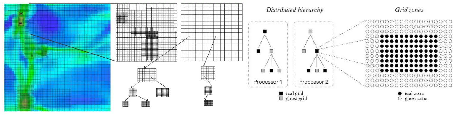
Fig 2 shows how ENZO runs it's simulations. The space is divided into grids where the physics is solved. Each grid is further subdivided into various zones which can then be stored on separate processors. The lower left panel depicts the hierarchy tree distributed across processors, distinguishing between Real Grids (data stored locally) and Ghost Grids (data stored on other processors). The right panel details an individual grid, showing the core Real Zones that contain active simulation fields surrounded by a layer of Ghost Zones used to exchange boundary information with neighbors via MPI.

The Simulation Suite

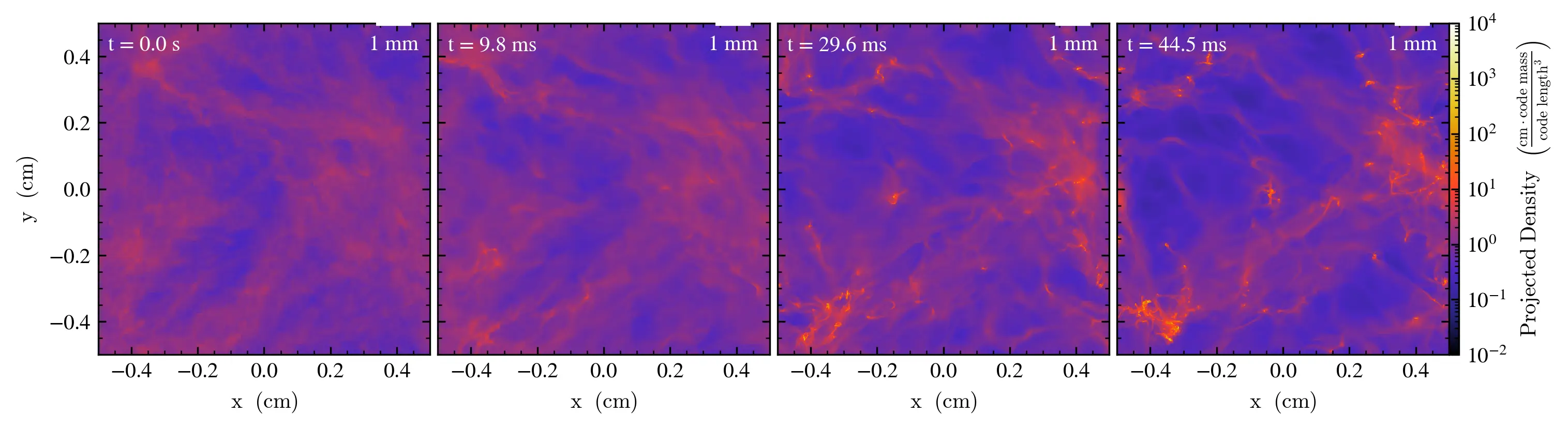
I generated a massive dataset of 3D volumetric snapshots. Below is a visualization of the full simulation suite, showing the density evolution over time as turbulence decays and gravity takes over.

3. The Solution: 3D Hybrid ConvGRU-UNet

Analyzing terabytes of 3D data by hand is impossible. Traditional threshold-based methods (like Clumpfind) are often too simplistic. I developed a Deep Learning approach to treat this as a spatiotemporal forecasting problem.

My model combines two powerful architectures:

• 3D U-Net: To extract spatial hierarchies and features (filaments, shocks) from the volumetric density field.
• ConvGRU (Convolutional Gated Recurrent Unit): To learn the time-evolution of these features. Unlike a standard RNN, a ConvGRU maintains the spatial structure of the memory.

Results & Performance

The model successfully predicts the location of sink particle formation N snapshots in advance. It learned to identify not just high-density regions, but converging flows, the velocity signatures that precede collapse.

Fig 4. The xy projection of density channel of model input and output.

By training on this synthetic data, we can potentially apply this model to real observational data cubes (like ALMA) to identify star-forming regions that are currently "quiet" but destined to collapse.

4. Some More Images :D :

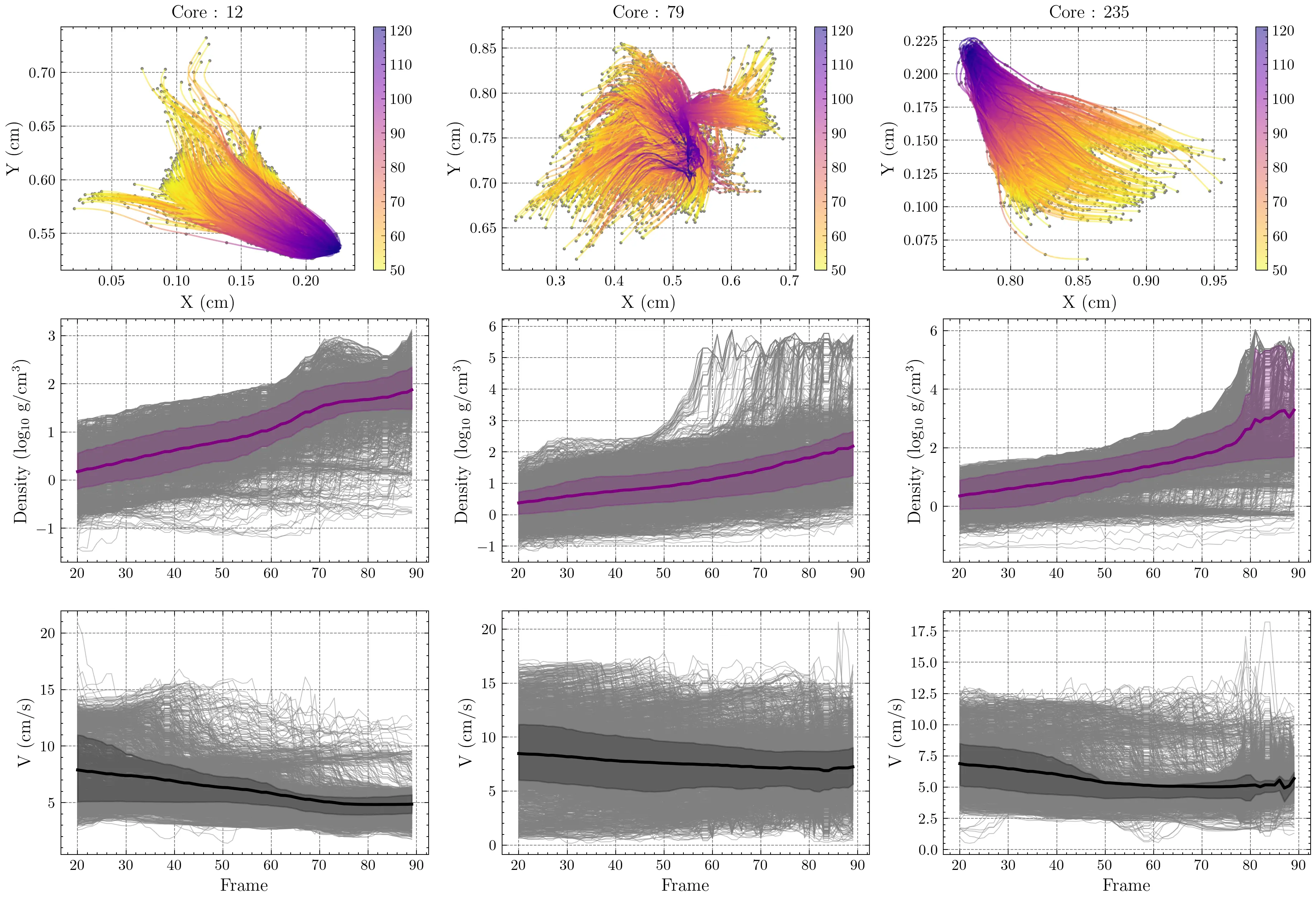
We also put Lagrangian tracer particles in our simulations that follow the flow of gas. We then go to the end of the simulation, identify prestellar cores, the tracers that belong to them and trace them back in time to see how they evolved. Fig 5 shows some visualizations of the core tracks and their features during collapse. Top row shows x-y projection of trajectories of tracer particles belonging to each core from the 50th (yellow) to the 120th (purple) frame. The middle row shows the density of the host cell of the tracers for the same time frame and the bottom row shows the velocity magnitude for each tracer during the collapse. For both \(rho\) and \(v\), we also show the median and the 25th-75th percentile region around the median. As the cores collapse, the density ramps up and there is relatively less dispersion of velocity.

Fig 5. Various features of 3 out of 285 cores in the simulation.

Here is a 2D xy density projection of 4 timesteps of a simulation showing the formation and collapse of a prestellar cores. We see the the filaments collapsing under gravity and forming dense cores that will eventually form stars.

Fig 6. 2D xy density projection of a simulation.